
Modular Vertical Farming in the UK

This page looks at the energy demand of our case studies and our process of modelling them along with potential changes.
Energy Modelling
Energy Demand & Offsetting (Introduction/Literature Review)
According to a report by WayBeyond & Agritecture, the high energy demand of vertical farms can be attributed to lighting and cooling consumption as shown in the Figure 1. This is true for the several types of vertical farm models included in the report that use controlled environments [1]. By using energy efficient equipment and using integrated renewable energy, the energy demand can be offset to make operations more sustainable and cost-effective [2][3].
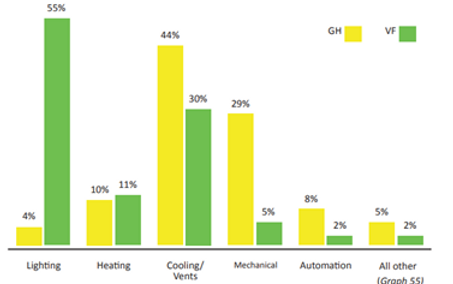
Figure 1. Sources of energy demand in greenhouses and vertical farms (WayBeyond & Agritecture, 2021)
Due to the modifiable characteristic of LEDs in terms of lighting spectrum and high lighting intensity available, it has been deemed viable to use it in indoor farming. However, vertical farms require high energy consumption due to the typical 16 hours running-time of lighting and the lighting energy intensity requirement of around 90W/m2 resulting to high heat gains[4][5].
In a study by Ahn et al. in 2015, the heat gain from LED lights can be calculated as 78.1% of its input power. This can be further reduced by removing heat through a heat exchanger with a factor between 86.5% and 98.1% [6]. Furthermore, while there are many passive cooling strategies for buildings, natural ventilation can effectively lower energy demand by removing the hot air inside the building and bringing fresh air inside to lower the temperature [7].
Methodology & Application
Model Description
The model’s dimensions were 11.84m x 2.273m x 2.121m, in line with research performed with a door on one wall of the container of dimensions 0.9m x 2.1m [8]. An image of the model can be found below.

Figure 2. Modular Vertical Farm
The one (1) zone model had heating and cooling active for all day types aiming for 20°C ambient room temperature for heating and cooling with a humidification range set for 55-65%. We then created an electrical network consisting of a PV panel, lighting and fans. We initially planned to model our offsetting assessment within ESP-r but later changed to PVSyst, however the system remained modelled.
The annual weather data from Dundee, UK (1980) was used to simulate the environmental conditions of the model with temperatures ranging from -6 to 24 ˚C.
Modelling Plan
The model started with collecting data from the industry stakeholders and then compiling them in Excel to determine the operational parameters needed to create our baseline model. After creating the initial model, the weather data in Dundee was used while changing the building properties in ESP-r to determine which will impact the overall energy demand of vertical farm. Finally, the simulated energy demand was used to calculate how much energy can be offset by the PV energy production modelled using PVSyst.
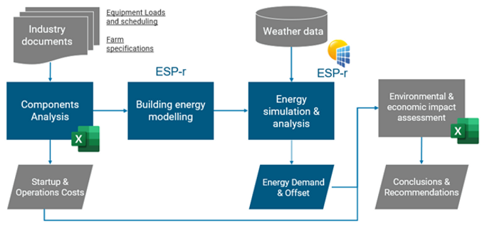
Figure 3. Energy Modelling Plan for Vertical Farm Setups
Modelling Parameters
The typical setup of the vertical farm is shown in Figure 4. For the model, we considered heating, cooling, insulation, lighting, and fans as the key components for simulation and analysis. All components with energy demand run for 24 hours in a day except for lighting which only runs for 16 hours. Since the CropBox model has more growing area, it requires a higher lighting requirement.
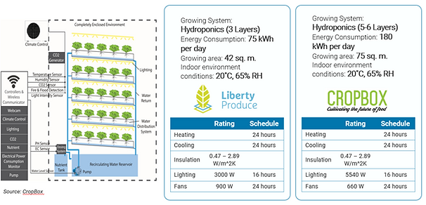
Figure 4. Vertical Farm Setup (left) and Modelling Parameters (right)
Energy Scenarios
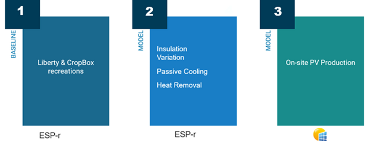
Figure 5. Energy Modelling Scenarios
Modelling Tools & Application
ESP-r
For the simulation of the first two energy scenarios, the Environmental Systems Performance – Research (ESP-r) modeling tool was used. This tool can conduct simulations and calculations to evaluate building performance [9].
Wall Insulation
There are four (4) different wall constructions used to assess the impact of insulation by recreating wall materials in ESP-r using known thicknesses and U-values shown in Table 1.
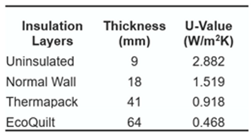
Table 1. Wall Insulation Properties
Heat Removal
To investigate the impact of changing the air inside the system, the value of air changes per hour (ACH) was changed between 1 and 10. Changing the air allows the replacement air inside the system with air outside, this is usually done to maintain air quality - in the case of this project, it was used to replace warm air with cooler air instead of simply cooling the air [10].
The heat gain for the LED lighting without and with cooling was computed using a factor a 0.781 and 0.21 of the power input to compare the impact on the cooling and overall energy demand of the system.
PVSyst & Energy Offsetting
PVSyst was used to model our electrical network to calculate PV output at our Dundee site location. Our aim was to determine the optimal setup to maximise energy exported from the panels, to see how much of our energy demand can be offset by onsite PV. The plane tilt was fixed and altered from 10° up to 45° was assessed, which was suggested by PVSyst to be the most optimised angle. As there were no constraints to the azimuth of the panels, the panels were assumed be south facing, to maximise their exposure to sunlight. No shading was also assumed, to allow a direct comparison of using traditional farmland for vertical farming setup. The area available for panels would be 27m2 , the area of the container. The PV panel used was the Jinkosolar JKM-420N-54HL4 and the inverter used is the PrimeVolt PV-5000S-HV. The area limit allowed for 14 panels to be used in the model. The value we used to determine to determine our energy output was the energy injected into the grid, as this showed us energy available after system and inverter losses.
The image below shows the interface for PVSyst for allowing alterations to the tilt and azimuth. It also shows that 45° tilt and 0 azimuth is the optimized variation because it has 0% loss with respect to optimum.
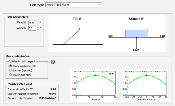
Figure 6. PVSyst Interface
Results & Analysis
Energy Demand
By assessing the annual energy demand of the models, it was determined that February is the month of least demand and August is the month of most demand. This aligns with stereotypical warmest/coolest UK months and further underlines the importance of reducing the required cooling as much as possible. For CropBox, the higher energy demand is mainly because of the higher lighting capacity, therefore, higher heat gains.

Figure 7. Annual Energy Demand of Liberty and CropBox Setups.
In both energy models, the major energy demand comes from lighting, fans, and cooling. This means that if the heat gained from the lights are reduced, the cooling and overall energy demand can be reduced significantly. Figure 8 below shows energy demand breakdown per demand source as a percentage of total demand for both setups. The graphs below are using Thermapack insulation with no additional cooling techniques.

Figure 8. Annual Energy Demand Breakdown of Liberty and CropBox Setups
Insulation
Using similar setups but altering the insulation of the model, it was determined in the Liberty model that poorer insulated models had a reduced energy demand, owing to a reduction cooling load. For Liberty, the cooling size remains between 3.5kW and 4kW throughout all variations however the required heating load almost tripled between Thermapack and EcoQuilt insulations, and uninsulated and normal wall insulations. The annual energy demand ranged between 34 to 41MWh annually. The best performing insulation was the normal wall model with an annual demand of 34.3MWh, 0.3MWh less than the uninsulated container.
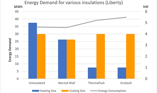
Figure 9. HVAC Energy Demand Compared to Equipment Size for Liberty
For CropBox’s energy demand, the same trend was observed for heating being greater for reduced insulation, 3kW for uninsulated and 3.5kW for normal wall compared to 1kW for Thermapack & EcoQuilt. The cooling load was 1kW higher for the Thermapack & EcoQuilt variations in comparison to uninsulated and normal walls. There is a greater required cooling size (5.5kW compared to 4kW) which again results in greater overall demand. Overall, energy demand varied from 49.7MWh to 62.3MWh annually, increasing as insulation quality improves.

Figure 10. HVAC Energy Demand Compared to Equipment Size for Cropbox
Heat Removal
The two graphs below show how ACH changes affected the demand for HVAC. These values are taken from using the Thermapack insulation as an example setup. Both liberty and CropBox show that total consumption falls slightly until 4 ACH occurs and then starts to increase again. Replacing the air leads to an increase in humidification and heating loads which ultimately minimize the potential for energy reduction to occur. Electrical load for lighting and fan remains constant in this setup so we plotted the consumption for HVAC & humidity instead of total demand. The HVAC & Humidity consumption for CropBox fell from 21.5MWh to 20.8MWh before slightly rising to 20.9MWh at 5 ACH’s then 23.4MWh at 10 ACH’s.
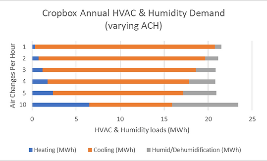
Figure 11. CropBox Annual HVAC Energy Demand
For the liberty model, HVAC & humidity consumption fell from 13.6MWh (1ACH) to 13.4MWh (4ACH) then increased again thereafter reaching 20.6MWh. This similarly showed a reduction until 4ACH but grew thereafter, showing further evidence for an optimal amount of air changes to reduce cooling.
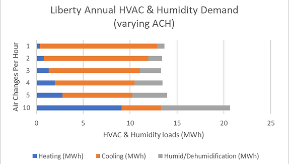
Figure 12. Liberty Annual HVAC Energy Demand
It was then assessed that the amount of reduction that could be done by using a heat exchange with air flow around the lighting to remove heat and thus reduce the heat irradiated into the container. The models showed an 18% reduction in energy usage for liberty and 24% reduction in CropBox.

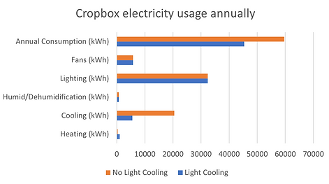
Figure 13. Liberty and CropBox Energy Demand with Heat Removal
Energy Offsetting
The simulated annual PV production after losses is 4707 and 5835 kWh for 0˚ and 45˚ tilt, respectively. This accounts for about 22% of Liberty’s annual consumption while only 9% for CropBox.
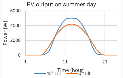
Figure 14. Power Output of the PV System during Summer and Winter day
Below is a graph assessing the monthly output for 10° angle tilts variations and 45° tilt.
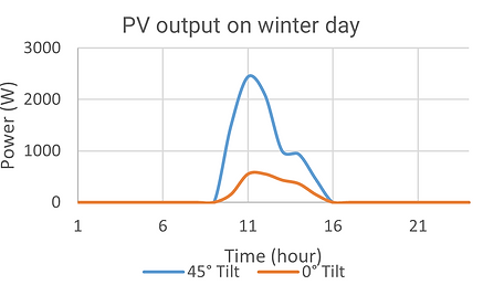

Figure 15. Annual PV Production with tilt variations
The graph above shows the output of the PV array at various angles over the course of the year. Ranging the tilt between 40-50 degrees. There was significant variations on output in winter months depending on the angle of tilt, with 66kWh in January at 0 tilt and 277kWh at 70 tilt, the highest output. Additionally, the optimized angle for May was 30 degree tilt and not 40 with the highest output. Further research should be done on the impact of maximizing solar output using a tracking PV system as it would be able to increase annual output further.
There is an opportunity to utilize all the energy generated from the system by moving the schedule of lighting earlier during the summer days since there is available energy produced as early as 7:00 AM. On the other hand, due to the lower solar irradiance levels during winter, all the energy produced is consumed by the energy demand. The maximum power output of the system reaches 5 kW during summer while the lowest is at 2.4 kW during winter.
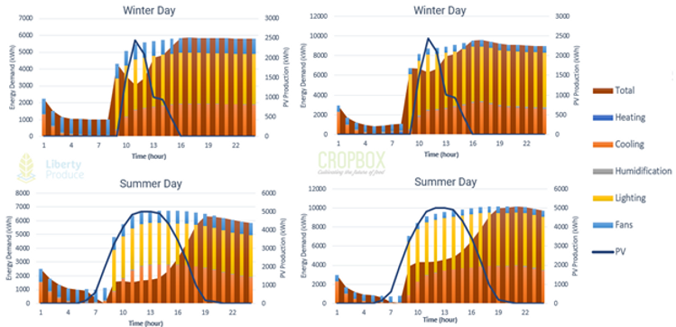
Figure 16. Energy Offset from PV Integration
Want to see more results? Download the models used here, and the results excel file here
References
[1] WayBeyond and Agritecture (2021). Global CEA Census Report WayBeyond. [online] Available at: https://engage.farmroad.io/hubfs/2021%20Global%20CEA%20Census%20Report.pdf [Accessed 7 May 2023].
[2] Al-Chalabi, M. (2015). Vertical farming: Skyscraper sustainability? Sustainable Cities and Society, 18(1), pp.74–77. doi:https://doi.org/10.1016/j.scs.2015.06.003.
[3] Teo, Y.L. and Go, Y. li (2021). Techno-economic-environmental analysis of solar/hybrid/storage for vertical farming system: A case study, Malaysia. Renewable Energy Focus, [online] 37, pp.50–67. doi:https://doi.org/10.1016/j.ref.2021.02.005.
[4] Nájera, C., Gallegos-Cedillo, V.M., Ros, M. and Pascual, J.A. (2022). LED Lighting in Vertical Farming Systems Enhances Bioactive Compounds and Productivity of Vegetables Crops. IECHo 2022. doi:https://doi.org/10.3390/iecho2022-12514.
[5] ifarm.fi. (n.d.). How Much Electricity Does a Vertical Farm Consume Using iFarm technologies? [online] Available at: https://ifarm.fi/blog/2020/12/how-much-electricity-does-a-vertical-farm-consume.
[6] Ahn, B.-L., Park, J.-W., Yoo, S., Kim, J., Leigh, S.-B. and Jang, C.-Y. (2015). Savings in Cooling Energy with a Thermal Management System for LED Lighting in Office Buildings. Energies, 8(7), pp.6658–6671. doi:https://doi.org/10.3390/en8076658.
[7] Taleb, H.M. (2014). Using passive cooling strategies to improve thermal performance and reduce energy consumption of residential buildings in U.A.E. buildings. Frontiers of Architectural Research, [online] 3(2), pp.154–165. doi:https://doi.org/10.1016/j.foar.2014.01.002.
[8] www.hgvalliance.com. (n.d.). Container Specifications | HGV Alliance UK Ltd. [online] Available at: https://www.hgvalliance.com/Container-Specifications [Accessed 9 May 2023].
[9] University of Strathclyde (n.d) Applications. Available at: https://www.esru.strath.ac.uk//applications/ [Accessed 28/04/2023]
[10] Wen, L. and Hiyama, K. (2018). Target Air Change Rate and Natural Ventilation Potential Maps for Assisting with Natural Ventilation Design During Early Design Stage in China. Sustainability, 10(5), p.1448. doi:https://doi.org/10.3390/su10051448.